Fusion Inside The Sun
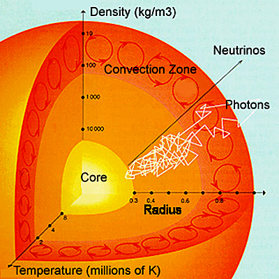
First, a quick review of how energy traverses the sun's regions. Nuclear fusion takes place in the sun's core. Energy then moves by photon radiation through the radiation zone (no fusion) to the convection zone. The energy in the form of heat then moves by convection to the surface. Convection is the flow of heat through a fluid, in this case plasma. (Convection does not occur in solids.) Convection takes place in one of two ways: by the random interaction of high energy (heated) particles (Brownian Motion) and by the flow of heated currents in the fluid plasma. Once the energy reaches the sun's surface it is mainly transmitted by rays (photons) and the solar wind (particles) to the rest of the the Heliosphere.
What exactly is fusion? Fusion is a process whereby 4 hydrogen nuclei at very high temperatures and pressure are burned into one helium nuclei plus some other particles and a lot of energy. The 4 hydrogen nuclei weigh more than the single helium nucleus and other particles. The balance of lost weight (mass) is converted into energy. In summary, the fusion process yields a helium nucleus, which contains 2 protons and 2 neutrons, plus 2 electrons plus 2 neutrinos and a lot of energy (photons). Because of Einstein's equation E=mc^2, a small amount of mass gets multiplied by the square of the speed of light (a very large number) resulting in a huge amount of energy being released from a very small amount of mass (similar to a nuclear bomb).
A huge number of neutrinos are also released by the fusion process. However, neutrinos rarely interact with other bits of matter. About a hundred billion neutrinos pass through your fingernails every second and we are completely unaware of them and they do no harm. A solar neutrino passing completely through the earth has about one chance in a thousand billion of being stopped by another particle. However, using 100,000 gallons of special fluids and very delicate sensing devices, neutrinos have been detected and measured. This experimental technique was used to verify the theory of nuclear fusion as the engine of energy in the core of our sun and other stars. Top
Coronal Loops
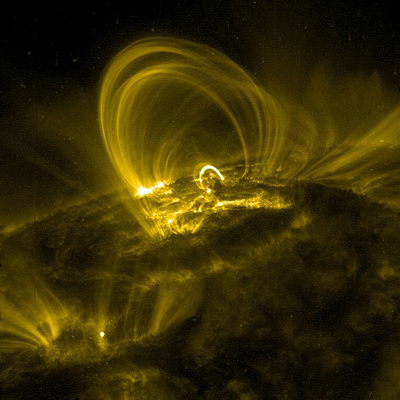
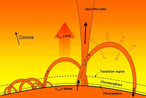
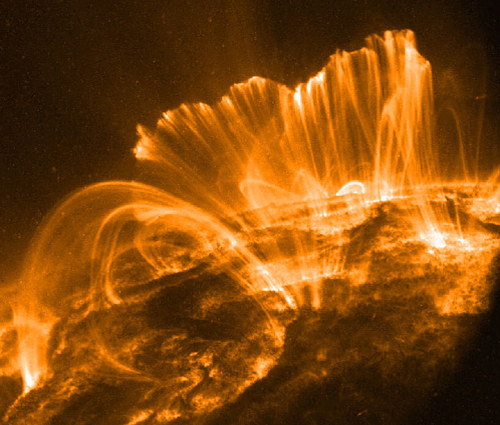
A coronal loop is a loop of magnetic flux filled with plasma anchored at both ends into the Photosphere and extending well into the Corona. Coronal loops come in many sizes. Some are quite small extending only into the Chromosphere 1,500 miles. Others extend well into the Corona and can be as high as 100,000 miles. See the diagram to the left and the one below.
One can mentally picture that underneath a coronal loop is a huge horseshoe magnet with a north and a south pole. The magnetic flux extends from one pole up into the Corona and then back down into the other pole. However, the coronal loops are dynamic. They can last anywhere from a day to months. They also get pushed around by the flow of the plasma. The number of coronal loops is directly linked to the solar cycle, i.e. when the sun is very active there are many coronal loops and vice versa. Coronal loops are often found with sunspots within their larger footprint.
Coronal loops have a wide variance in their energy and temperatures. Those under one million degrees Kelvin (1 MK) are referred to as cool loops. Those around 1MK are warm loops and those over 1MK are called hot loops. The different categories produce radiation of different wavelengths.
How do the coronal magnetic loop fields form?
Just beneath the surface of the Photosphere there are small scale magnetic fields forming all the time. These local fields form a thick carpet-like surface of revolving plasma currents circulating in small vertical loops as the heat from the radiation zone makes its way to the surface through the convection zone.
Separately there are also large currents flowing from the poles deep underneath the surface to the equator, then up to the surface and back again to the poles, referred to as the sun's Conveyor Belts. In addition, the convection zone is rotating, but in a "differential" way. Meaning the plasma at the equator is rotating faster than the plasma at the poles thus causing many shears in the east-west flow from the equator to the poles.
So we have three conflicting plasma flows: vertical loops from the bottom of the convection floor to the surface, north-south conveyor belts, and east-west rotational shears. This results in the various magnetic fields becoming tangled and twisted causing a build up of stored magnetic energy. At some point there is a release of this magnetic energy as the magnetic fields re-configure themselves into a lower energy state and the excess energy is converted into kinetic and thermal energy. See the "Magnetic Reconnection" section below this one. This results in an ejection of plasma into the corona as the plasma follows the new magnetic field lines. Some ejections are bigger than others causing the coronal loops to be of different sizes.
At the poles a slightly different phenomenon takes place. Instead of the loops being closed, most of them are open and for an extended period of time. In this case the plasma is shot out into outer space and forms the "fast" solar wind. Top
Magnetic Reconnection
Solar magnetic reconnection is a physical process in highly conductive plasmas where magnetic fields clash, re-configure themselves into a lower energy level, and the excess magnetic energy is then converted into kinetic and thermal energy.
On the sun this results in the creation of huge solar flares that are equivalent to billions of megatons of TNT exploding within a few seconds. Electrons and other particles that are accelerated by magnetic reconnection in a solar flare approach the speed of light. Closer to home, the Northern Lights are an example of magnetic reconnection in the earth's atmosphere.
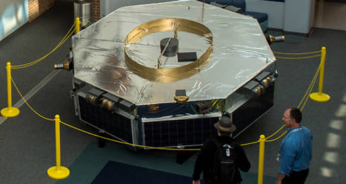
NASA has launched a special mission to get to the bottom of the magnetic reconnection mystery. It's called MMS, short for "Magnetospheric Multiscale". See the NASA picture above of one of the four spacecraft. Each one is shaped like a giant hockey puck, about four meters in diameter and one meter in height. In space, however, they are much larger when their sensors are extended.
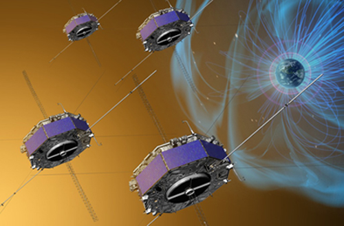
The four spacecraft were designed, built and tested at NASA’s Goddard Space Flight Center and launched on March 12th, 2015. See a NASA artist's conception of the four satellites in space to the left. The four spacecraft will fly through the earth's magnetic field (the magnetosphere) to study "reconnections" with the magnetic field of the sun.
Within the huge magnetic bubble that surrounds our planet, the reconnection process plays out over tens of miles in several directions.
"After launch, the spinning spacecraft unfurled their electromagnetic sensors, which are at the end of wire booms about 180 feet long," says Craig Tooley, MMS Project Manager at Goddard.
"When fully extended, these sensors are as big as a baseball field." These sprawling, spinning probes fly in precise formation, about 6 miles (10 km) apart and are guided by GPS satellites orbiting earth far below them.
MMS will fly directly into a reconnection zone. The spacecraft are built sturdy enough to withstand the reconnection events known to occur in earth's magnetosphere. "One of the mysteries of magnetic reconnection is why it’s explosive in some cases, steady in others, and in some cases magnetic reconnection does not occur at all," said Tom Moore, the mission scientist for MMS at NASA's Goddard.
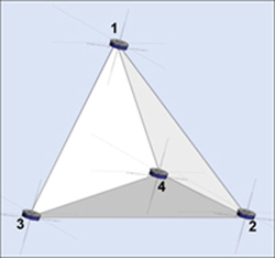
The four MMS spacecraft fly in a full pyramid formation to create a 3-D map of any phenomena they observe. See the pyramid sketch to the left illustrating how MMS captures 3-D data.
On October 16, 2015, the spacecraft traveled right through a magnetic reconnection event at the boundary where earth’s magnetic field bumps up against the sun’s magnetic field. In only a few seconds, the 25 sensors on each of the spacecraft collected thousands of observations. This opened the door for scientists to track how the magnetic and electric fields changed, as well as the speeds and direction of the various charged particles.
As the four spacecraft flew across the magnetosphere's boundary they flew directly through the "dissipation region" where the magnetic reconnection occurred. The spacecrafts were able to track exactly how the magnetic fields suddenly shifted and also how the electron particles flew away.
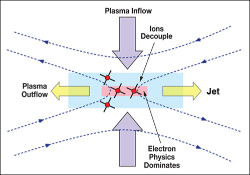
See the illustration to the left. The purple arrows represent the magnetic fields of the earth and sun coming together. The yellow arrows indicate the mass flow of electrons "after" the reconnection.
"The data showed the entire process of magnetic reconnection to be fairly orderly and elegant," said Michael Hesse, a space scientist at Goddard. "There doesn't seem to be much turbulence present, or at least not enough to disrupt or complicate the process."
Spotting the characteristic "crescent shape" in the electron distributions suggests that it is the physics of electrons that is at the heart of how magnetic field lines accelerate the particles.
The data shows that electrons shoot straight away from the original event at hundreds of miles per second crossing the magnetic boundaries that would normally deflect them. Once across the boundary, the particles curve about 90 degrees in response to the new magnetic fields they encounter. These observations align with a computer simulation known as the crescent model, named for the characteristic "crescent shapes" that the plots show to represent the electrons new paths.
Since its first direct observation of a magnetic reconnection, as of May 2016 MMS has flown through similar events five more times, providing more detailed information about this fundamental process. For a NASA 2 minute video on MMS click here.
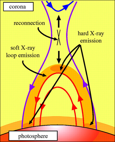
Solar Flares. To the left is an example of magnetic reconnection on the sun resulting in a sun flare. The purple lines represent the two magnetic field lines about to crash at point "X". At the flare itself, there are three points of very hard X-ray emissions (greater than 10 keV) located at the two bottoms of the flare and one at the peak. In between there are soft X-rays. Above the reconnection point there are more magnetic lines, but nothing visible to the eye.
Flares produce radiation across the electromagnetic spectrum, although with different intensities. Most of their energy goes to frequencies outside of our visual range so the majority of flares are not visible to the naked eye and must be observed using special instruments. While not very intense at normal visible light, they can be very bright at particular frequencies.
Some flares are followed by a Coronal Mass Ejection (CME), an unusually large release of plasma from the solar corona. CMEs often follow solar flares releasing their plasma into the solar wind. The energy emitted from a flare is about one sixth of the sun's total energy output each second. For more info on solar flares click here.
Magnetohydrodynamics - MHD. MHD is the study of the "magnetic properties" of electrically conducting fluids such as salt water, liquid metals, electrolytes and plasmas.
The word magnetohydrodynamics is derived from magneto meaning magnetic field, hydro meaning water, and dynamics meaning motion.
The sun is all plasma, hence MHD is the technology used when scientists simulate sun events. The fundamental concept behind MHD is that magnetic fields induce currents in a moving conductive fluid, which in turn polarizes the fluid, and induces major changes in the magnetic field itself. The differential equations involved must be solved simultaneously and make for quite difficult mathematics.
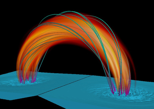
The image to the left is from an MHD simulation of a sun flare from the University of Palermo in Buenos Aires, Argentina. The project investigates the heating released by the magnetic reconnection of a twisted coronal loop. Top
Solar Spicules
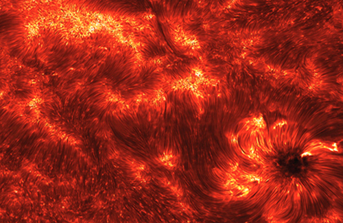
Spicules (spik'-cules) are the dark red images in the picture to the left. The spikes of superheated gas are small compared to many of the sun's prominent features, such as giant loops that are flung thousands of miles into the solar corona. The spicules are a relatively small 300 miles in diameter and typically shoot a relatively modest 3,000 to 6,000 miles above the sun's surface. (Large solar flares can reach up to 100,000 miles above the sun's surface.)
Spicules scream upward at 150,000 mph (Wow!) and then vanish within minutes, making them hard to study. A close up view to the left from the Solar Dynamics Observatory (SDO) spacecraft using ultraviolet technology shows the dark red Spicules.
At any one time there are about 100,000 active Spicules on the sun's surface. They are found in regions of strong magnetic fields. Spicules live for about 5 minutes. The key to their origin is the regular cycle with which spicules regenerate. Every five minutes or so, one leaps forth from the same spot. NASA compares the Spicules to "seaweed" in the ocean swaying back and forth in the ocean's waves. Magnetic fields, called "Alfvén Waves", ripple inside the Spicules causing them them to sway like seaweed. Top
Alfvén Waves
Alfvén Waves, named after Hannes Alfvén, are magnetically induced waves in electrically conducting fluids. Conducting fluid examples are salt water, electrolytes, liquid metals, and of course plasmas. Alfvén discovered this phenomenon in 1942 and won the Nobel Prize in Physics for it in 1970.
Alfvén suggested that large plasmas could carry huge electric currents capable of generating "galactic magnetic fields" (i.e. possibly the solar wind's Magnetic Current Sheet).
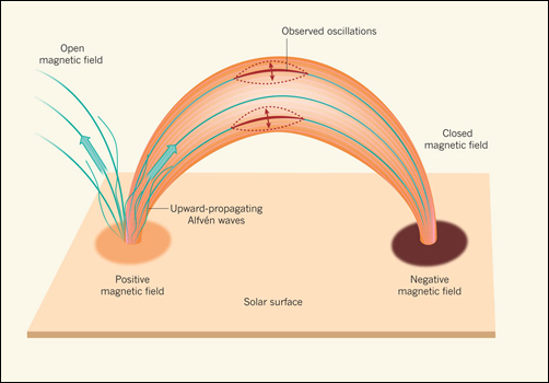
Alfvén Waves travel up and down a magnetic field much the same way a sound wave travels up and down a plucked guitar string. See the solar magnetic field illustrated to the left which contains Alfvén magnetic waves flowing through it from the positive origination spot to the negative destination. It appears the Alfvén waves are intrinsically involved as they “ride” the spicules, driving up heat energy in the spicule plasma to extreme Coronal temperatures.
NASA's SDO is now able to measure how much energy is carried by the Alfvén Waves spewing out from the jets of Spicules. Recent research shows that the Alfvén waves carry 100 times more energy than previously thought.
See the actual photo to the left of some solar Alfvén Waves taken by SDO at infrared frequencies. The Alfvén Waves carry enough energy to drive the intense heat of the Corona to 200 to 400 times hotter than the sun's surface and the solar winds up to 1.5 million miles per hour. Whether or not all this energy is actually transferred into heat is not known at the moment.
The Alfvénic Waves as we know them today could account for the energy of the Corona and Solar Wind, but there is not enough energy to account for the huge mass of plasma materials ejected during Coronal Mass Ejections (CMEs). Although the wave generation process may sound fairly straightforward, how the energy passes from the waves to the plasma is not understood.
Scott McIntosh at the National Center for Atmospheric Research (NCAR) in Boulder, Colorado says, "We still don't perfectly understand the process going on, but we're getting better and better observations. The next step is for people to improve the theories and models to really capture the essence of the physics that's happening. Now that the real power of the waves has been revealed in the Corona, the next step in unraveling the mystery of its extreme heat is to study how the waves transfer their energy to the plasma." Top
The Solar Wind
The Solar Wind is a constant stream of charged particles in all directions emanating from the sun's extremely hot outer atmosphere (the Corona). At these extremely hot levels, the sun's gravity can't hold on to the rapidly moving particles, and they stream away from the star, never to return. The solar wind can be thought of as an extension of the Corona into interplanetary space. The Corona does not have a pronounced upper edge.
The glow of the Corona is a million times less bright than the Photosphere, so it can only be seen when the central disk of the sun is blocked out by an instrument called a "coronagraph". See the photo to the left. The Corona is 10 billion times less dense than the sea level atmosphere of the earth.
The Corona is 5,800 K degrees at the sun's surface, but up to 20,000,000 K (i.e. 20 million K) at its outermost hottest locations! It is not clear at this time how to explain these extreme outer Corona temperatures, but they certainly contribute to the solar wind.
In 1910 British astrophysicist Arthur Eddington suggested the existence of the solar wind without naming it. He postulated that the ejected sun material consisted of electrons, while in another study he suggested them to be ions. However, the idea never fully caught on.
The first person to suggest that they were both electrons and ions was Norwegian physicist Kristian Birkeland. His geo-magnetic surveys showed that the northern aurora activity (northern lights) was almost never interrupted.
As the displays were being produced by particles from the sun, he concluded that the earth was being continually bombarded by "rays of electric corpuscles emitted by the sun".
The sun's activity shifts over the course of its eleven year cycle. The sun spot numbers, radiation levels, and amount of ejected material all vary over time. These alterations affect the solar wind including its magnetic field properties, velocity, temperature and density.
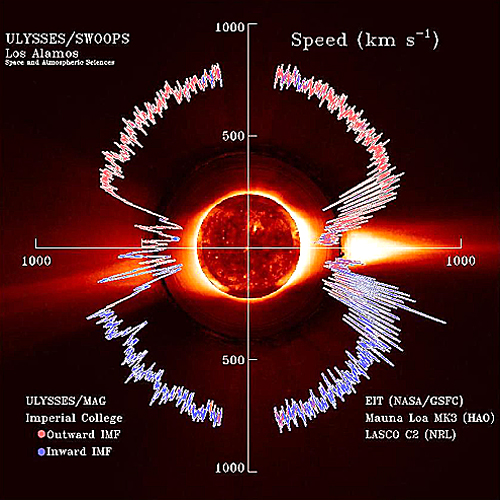
The solar wind also differs depending on which part of the sun it originates from and how quickly that portion is rotating. See the wind speed chart to the left.
The solar wind has two components - the "slow" wind and the "fast" wind. The slow wind travels about 200 miles/second (300 km/sec.), whereas the fast wind travels about 500 miles a second (800 km/sec.).
The slow solar wind originates from a region around the sun's equator that is known as the "streamer belt". At the streamer belt, the solar wind emanates more slowly and the temperatures in the slow wind are hotter reaching up to 1.6 million degrees C.
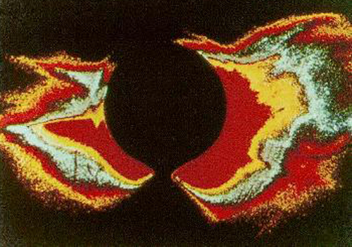
See the x-ray image of the sun's magnetic fields to the left. In the streamer belt the magnetic field lines close in on themselves, particularly in periods of low solar activity.
These closed field lines trap the hot coronal gases, leading to enhanced x-ray emissions from these hotter regions, but at the same time they suppress the contribution to the solar wind.
The solar wind contributes a mass loss of the sun of more than 1 million tons of material per second. This is equivalent to the sun losing the the size of the earth every 150 million years.
However this is insignificant, only about 0.01% of the sun's total mass has ever been lost due to the solar wind.
The solar wind keeps traveling at about a million miles per hour for about a year until it finally reaches the edge of the Heliosphere and mixes with cosmic rays from far outer space.
See theHeliosphere Page for more outer space information. Top
Coronal Holes
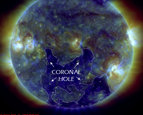
The "fast" solar wind originates from Coronal holes which are funnel-like regions of open magnetic field lines mostly close to the sun's poles. The "fast" solar wind is a little over twice the speed of the "slow" solar wind.
See the Coronal hole picture to the left taken by NASA's Solar Dynamics Observatory on October 13, 2016. It shows the dark Coronal hole pointing almost directly at the earth.
Coronal holes are places in the sun's atmosphere where the magnetic field opens up and allows normally-trapped solar wind to escape.
The Coronal hole pictured at the left is broad, and the stream of solar wind it spit out influenced the earth's atmosphere for several days.
The aurora borealis seen at the northern and southern poles are the results of the solar wind entering the earth’s atmosphere.
Coronal holes are part of the sun's magnetic field that arches away from areas in the Corona that are very thin due to lower levels of energy and gas. These lower energy levels cause Coronal holes to develop if the magnetic lines are not closed.
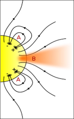
See the magnetic line diagram of the sun to the left. In the 'A' sections the magnetic lines are closed causing normal solar flares and CMEs to develop. In the 'B' area the magnetic lines are open and the solar wind escapes into interplanetary space. As the solar wind escapes, it leaves behind a lower density and lower solar temperature area.
The size and population of Coronal holes vary based on the solar cycle. It is known that every 11 years Coronal holes are at their minimum. During a solar maximum, the number of Coronal holes actually decreases because the magnetic fields are about to reverse in the sun’s core. New Coronal holes appear at the opposite magnetic alignment. They develop and expand over the poles and remain active at the poles even when the sun moves back to a solar maximum.
Coronal holes are linked to concentrations of open magnetic field lines. During the solar minimum, Coronal holes are mainly found at the sun's polar regions, but they can be located anywhere on the sun during a solar maximum. There are permanent Coronal holes at the north and south poles of the sun. These permanent polar holes reach their largest size when total activity on the sun is at its minimum.
Since Coronal holes are regions in the sun’s Corona that have much lower densities and temperatures than most of the Corona, these regions are very thin. Since these areas are so thin, particles within the Chromosphere can easily break through the magnetic field lines and escape. Temperatures in the fast wind reach up to 800,000 degrees C.
The fast solar wind is made up of electrons and nuclei of hydrogen and helium as well as other particles such as ions and more massive atoms that include silicon, sulfur, calcium, chromium, nickel, iron, and argon. A typical fast wind storm contains about 10^9 kilograms of material. Top
A Spacecraft Into The Sun
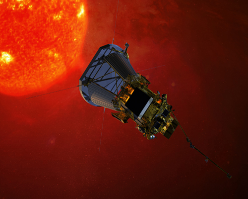
Why the sun's atmosphere is up to 450 times hotter than its surface has been a long standing physics mystery of the sun. A NASA spacecraft, the Parker Solar Probe (formerly the Solar Probe Plus) scheduled to launch in July, 2018, has been designed to gain some insight.
Scientists at Johns Hopkins University in Baltimore developed the Parker Solar Probe, named after Eugene Parker, the first person to predict the existence of the supersonic solar wind. (Eugene Parker is a 90 year old professor emeritus from the University of Chicago, the first living person to have a spacecraft named after him.)
By flying into the sun’s outer atmosphere, the Parker Solar Probe will gather data on the processes that "heat the corona" and "accelerate the solar wind" - the two fundamental mysteries that have been top priority science goals for decades. The Parker Solar Probe will carry 10 instruments specifically designed to help solve the two key puzzles of solar physics.
Eight weeks after launch, The Parker Solar Probe will arrive at the sun to begin the first of 24 sun orbits plus 7 flybys of Venus to gradually shrink its distance to the sun. Eventually, it will come as close as 3.9 million miles, which is seven times closer than any previous spacecraft. (Earth’s average distance to the sun is 93 million miles.)
At its closest approach, the Parker Solar Probe will zip past the sun at 430,000 miles per hour, protected by a carbon-composite heat shield that must withstand up to 2,500 degrees Fahrenheit and survive blasts of radiation not experienced by any previous spacecraft. Engineers have also built and tested a liquid-cooling system to keep the spacecraft’s solar arrays at a safe operating temperature throughout the voyage.
“The Parker Solar Probe will fly closer to the sun than any spacecraft before it, almost 10 times closer to the sun than the planet Mercury, and this presents unprecedented technical challenges,” says Andy Driesman, the Parker Solar Probe Project Manager. “Whether it was devising ways for a spacecraft to survive so close to the sun, or to collect data in such an extreme environment, the concept of an operational solar probe has challenged engineers and scientists for decades."
The Parker Solar Probe, which cost more than $1 billion, was initially planned to be launched in 2015. However, the launch date was bumped to the middle of 2018 to spread out the cost. Top
The Ultimate Space Power Station
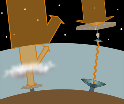
Space Based Solar Power (SBSP) The ultimate solar power station is in outer space. As shown on the left hand side in the sketch at the left, there are energy losses as the sun's rays are reflected from the atmosphere, clouds, dust, the day-night cycle and seasonal changes. Only about 50% of the sun's energy reaches the earth and then only 15% to 25% of that reaches the grid.
As shown on the right hand side of the sketch, a SBSP system would collect solar energy by a satellite 24 hours a day, convert it to microwaves, transmit the microwave radiation to earth where it would be captured by a very large ground antenna and converted into usable electricity on the grid. The energy efficiency from the space station to the grid would be about 50%, roughly the same as fossil fuel electrical plants.
The SBSP concept was first published in November 1968 by Peter Glaser and in 1973 he was granted a U.S. patent for his method of transmitting power from a satellite using microwaves sent from a large antenna to a combination rectifier-antenna, now called a "rectenna" on the ground.
NASA began to study the concept in 1974. They found that while the concept had several major problems (the expense of putting the solar satellite in orbit and the lack of experience for projects of this scale in space) it showed enough promise to merit further research. Research has continued to this day.
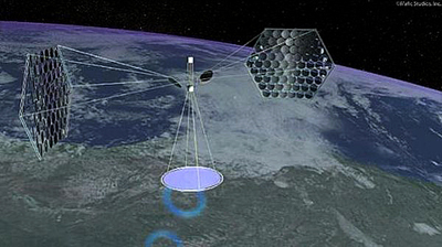
There have been enormous improvements in solar panel efficiency reducing the size of the panel array in space. (See an artist's sketch of a proposed satellite system at the left.) Rocketry has also improved, but not sufficiently enough that "hundreds of transport trips" can be undertaken cost effectively at this time.
Satellite transportation costs remain the biggest obstacle to this technology being implemented. Many noted scientists believe that if the US "concentrated" on this effort, the costs of transporting the spacecraft materials to space would come down and the whole project would be cost competitive with fossil fuels.
Let there be no question, that as we come to the later part of the 21st century and with the availability of fossil fuels declining, resulting in extremely high fuel prices, SBSP will be seen as the ultimate answer. The real question is "Will we by then be ready to exploit this endless source of cheap electrical power?" For a more detailed discussion of SBSP see the Solar High Brochure and Web Site by Dr. Philip Chapman former NASA Astronaut, Physics Professor at MIT, and Employee of Dr. Peter Glaser. For a very interesting NASA video featuring a commentary by Dr. Peter Glaser himself click here.
Top